16. Analysis of contingency tables#
本节需要的包:
require(s20x)
Show code cell output
Loading required package: s20x
16.1. Introduction#
分类统计表
AP.df <- read.table("../data/AttendPass.txt", header = T)
head(AP.df, 8)
| Subject | Pass | Attend | |
|---|---|---|---|
| <int> | <chr> | <chr> | |
| 1 | 1 | pass | attend |
| 2 | 2 | pass | attend |
| 3 | 3 | pass | attend |
| 4 | 4 | pass | attend |
| 5 | 5 | pass | attend |
| 6 | 6 | fail | not.attend |
| 7 | 7 | pass | not.attend |
| 8 | 8 | fail | attend |
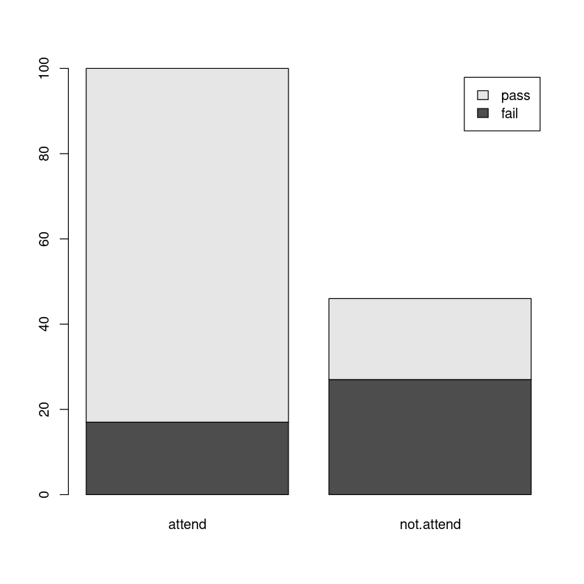
AP.tbl <- with(AP.df, table(Attend, Pass))
AP.tbl
            Pass
Attend       fail pass
  attend       17   83
  not.attend   27   19
plot(AP.tbl, main = "", las = 1)

barplot(t(AP.tbl), legend = T)
16.2. The binomial approach to contingency table analysis#
Freqs.df <- data.frame(
    Attend = c("not.attend", "attend"),
    Fail = c(27, 17), Pass = c(19, 83)
)
Freqs.df <- transform(Freqs.df, Attend = factor(Attend))
Freqs.df
| Attend | Fail | Pass |
|---|---|---|
| <fct> | <dbl> | <dbl> |
| not.attend | 27 | 19 |
| attend | 17 | 83 |
AP.binom <- glm(cbind(Pass, Fail) ~ Attend, data = Freqs.df, family = binomial)
summary(AP.binom)
Call:
glm(formula = cbind(Pass, Fail) ~ Attend, family = binomial,
    data = Freqs.df)

Deviance Residuals:
[1]  0  0

Coefficients:
                 Estimate Std. Error z value Pr(>|z|)
(Intercept)        1.5856     0.2662   5.956 2.58e-09 ***
Attendnot.attend  -1.9370     0.4007  -4.834 1.34e-06 ***
---
Signif. codes:  0 ‘***’ 0.001 ‘**’ 0.01 ‘*’ 0.05 ‘.’ 0.1 ‘ ’ 1

(Dispersion parameter for binomial family taken to be 1)

    Null deviance:  2.5162e+01  on 1  degrees of freedom
Residual deviance: -3.5527e-15  on 0  degrees of freedom
AIC: 12.756

Number of Fisher Scoring iterations: 3
exp(confint(AP.binom))[2, ]
Waiting for profiling to be done...
- 2.5 %
- 0.0642983964738621
- 97.5 %
- 0.311134072466483
16.3. The Poisson approach to contingency table analysis#
library(dplyr)
AP.df <- read.table("../data/AttendPass.txt", header = T)
AP.df <- transform(AP.df, Pass = factor(Pass), Attend = factor(Attend))
Freqs2.df <- AP.df %>%
    group_by(Attend, Pass) %>%
    summarize(freq = n()) %>%
    data.frame()
Freqs2.df
Error in library(dplyr): there is no package called ‘dplyr’
Traceback:

1. library(dplyr)
Freqs2.df$Attend <- relevel(Freqs2.df$Attend, ref = "not.attend")
AP.pois <- glm(freq ~ Attend * Pass, family = poisson, data = Freqs2.df)
summary(AP.pois)
| Estimate | Std. Error | z value | Pr(>|z|) | |
|---|---|---|---|---|
| (Intercept) | 3.2958369 | 0.1924501 | 17.125671 | 9.550242e-66 |
| Attendattend | -0.4626235 | 0.3096136 | -1.494197 | 1.351243e-01 |
| Passpass | -0.3513979 | 0.2994472 | -1.173489 | 2.405999e-01 |
| Attendattend:Passpass | 1.9370252 | 0.4006749 | 4.834407 | 1.335434e-06 |
Attendattend:Passpass: 6.93808049535602
Null deviance 叫做零模型自由度,Residual deviance 叫做残差自由度。
残差自由度等于零时,参数个数等于该数据的行数。由此可以推出原数据有 4 行。
exp(confint(AP.pois))[4, ]
Waiting for profiling to be done...
- 2.5 %
- 3.21404850350281
- 97.5 %
- 15.552487384471
16.4. Equivalence of the binomial and Poisson approaches#
Freqs.df
exp(confint(AP.pois))[4, ]
| Attend | Fail | Pass |
|---|---|---|
| <fct> | <dbl> | <dbl> |
| not.attend | 27 | 19 |
| attend | 17 | 83 |
Waiting for profiling to be done...
- 2.5 %
- 3.21404850350281
- 97.5 %
- 15.552487384471
predict(AP.pois, type = "response")
- 1
- 17.0000000000001
- 2
- 83.0000000000001
- 3
- 27
- 4
- 19
Freqs.df
coef(summary(AP.pois))
exp(coef(AP.pois))[4]
| Attend | Fail | Pass |
|---|---|---|
| <fct> | <dbl> | <dbl> |
| not.attend | 27 | 19 |
| attend | 17 | 83 |
| Estimate | Std. Error | z value | Pr(>|z|) | |
|---|---|---|---|---|
| (Intercept) | 3.2958369 | 0.1924501 | 17.125671 | 9.550242e-66 |
| Attendattend | -0.4626235 | 0.3096136 | -1.494197 | 1.351243e-01 |
| Passpass | -0.3513979 | 0.2994472 | -1.173489 | 2.405999e-01 |
| Attendattend:Passpass | 1.9370252 | 0.4006749 | 4.834407 | 1.335434e-06 |
Attendattend:Passpass: 6.93808049535602
options(digits = 4)
OR <- 27 * 83 / (17 * 19)
OR