14. Poisson modelling of count data: Two examples#
本节需要的包:
require(s20x)
Show code cell output
载入需要的程辑包:s20x

Warning message:
"程辑包's20x'是用R版本4.2.3 来建造的"
14.1. Example 1: Earthquake frequency#
古腾堡•里希特定律说,在一定时期内,预期的地震数量会随着地震的大小而成倍地减少。其公式为:
\[
\log_{10}N=a-bM
\]
where N is the expected number of earthquakes of magnitude M or more on the Richter scale. Here, a and b are unknown parameters. 其中N是里氏震级M级以上的地震的预期数量。这里,a和b是未知参数。
Quakes.df <- read.table("../data/EarthquakeMagnitudes.txt", header = TRUE)
Quakes.df$Locn <- as.factor(Quakes.df$Locn)
# Print first 4 SC observations
subset(Quakes.df, subset = c(Locn == "SC"))[1:4, ]
# Print first 4 WA observations
subset(Quakes.df, subset = c(Locn == "WA"))[1:4, ]
| Locn | Magnitude | Freq | |
|---|---|---|---|
| <fct> | <dbl> | <int> | |
| 1 | SC | 5.25 | 32 |
| 2 | SC | 5.50 | 27 |
| 3 | SC | 5.75 | 10 |
| 4 | SC | 6.00 | 9 |
| Locn | Magnitude | Freq | |
|---|---|---|---|
| <fct> | <dbl> | <int> | |
| 10 | WA | 5.25 | 13 |
| 11 | WA | 5.50 | 6 |
| 12 | WA | 5.75 | 2 |
| 13 | WA | 6.00 | 1 |
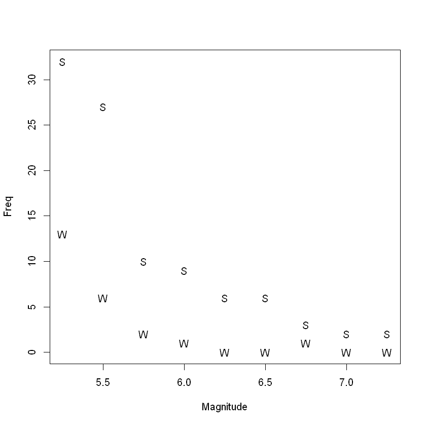
plot(Freq ~ Magnitude, data = Quakes.df, pch = substr(Locn, 1, 1))
Quake.gfit <- glm(
Freq ~ Locn * Magnitude,
family = poisson,
data = Quakes.df
)
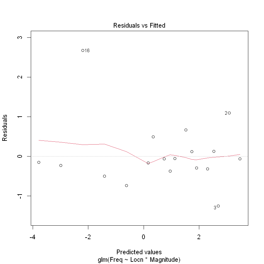
plot(Quake.gfit, which = 1)
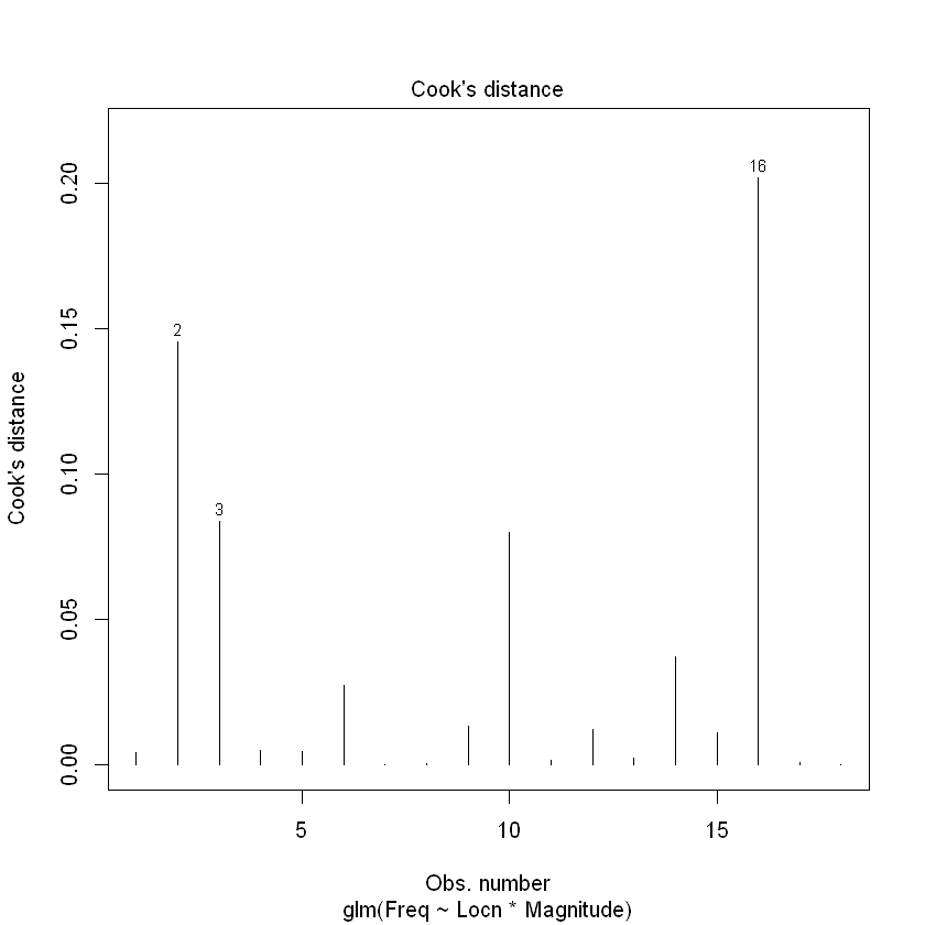
plot(Quake.gfit, which = 4)
summary(Quake.gfit)
Call:
glm(formula = Freq ~ Locn * Magnitude, family = poisson, data = Quakes.df)

Deviance Residuals:
    Min       1Q   Median       3Q      Max
-1.3261  -0.3225  -0.1172   0.1241   1.6190

Coefficients:
                 Estimate Std. Error z value Pr(>|z|)
(Intercept)       11.6923     1.1762   9.941  < 2e-16 ***
LocnWA             7.3923     3.9500   1.871   0.0613 .
Magnitude         -1.5648     0.2055  -7.616 2.61e-14 ***
LocnWA:Magnitude  -1.5884     0.7199  -2.206   0.0274 *
---
Signif. codes:  0 '***' 0.001 '**' 0.01 '*' 0.05 '.' 0.1 ' ' 1

(Dispersion parameter for poisson family taken to be 1)

    Null deviance: 176.1767  on 17  degrees of freedom
Residual deviance:   8.2295  on 14  degrees of freedom
AIC: 65.11

Number of Fisher Scoring iterations: 5
1 - pchisq(8.23, 14)
0.877002515280767
Quake.cis <- confint(Quake.gfit)
exp(Quake.cis[3, ])
## To interpret as percentage decreases
100 * (1 - exp(Quake.cis[3, ]))
Waiting for profiling to be done...
- 2.5 %
- 0.137474251413585
- 97.5 %
- 0.308243734868518
- 2.5 %
- 86.2525748586415
- 97.5 %
- 69.1756265131482
Quakes.df$Locn2 <- factor(Quakes.df$Locn, levels = c("WA", "SC"))

Quake2.gfit <- glm(Freq ~ Locn2 * Magnitude, family = poisson, data = Quakes.df)
(Quake.WA.ci <- exp(confint(Quake2.gfit)[3, ]))

## To interpret as percentage decreases
100 * (1 - Quake.WA.ci)
Waiting for profiling to be done...
- 2.5 %
- 0.00907766110939229
- 97.5 %
- 0.140175444866894
- 2.5 %
- 99.0922338890608
- 97.5 %
- 85.9824555133106
14.2. Example 2: Snapper counts in and around marine reserves#
Snap.df <- read.table("../data/SnapperCROPvsHAHEI.txt", header = TRUE)
with(Snap.df, {
    Locn <- as.factor(Locn)
    Reserve <- as.factor(Reserve)
})
Snap.df
| Locn | Reserve | Freq |
|---|---|---|
| <chr> | <chr> | <int> |
| Leigh | N | 2 |
| Leigh | N | 1 |
| Leigh | N | 0 |
| Leigh | Y | 5 |
| Leigh | Y | 11 |
| Leigh | Y | 7 |
| Leigh | Y | 8 |
| Leigh | Y | 7 |
| Leigh | Y | 14 |
| Hahei | N | 1 |
| Hahei | N | 0 |
| Hahei | N | 1 |
| Hahei | N | 0 |
| Hahei | Y | 3 |
| Hahei | Y | 2 |
| Hahei | Y | 1 |
| Hahei | Y | 5 |
| Hahei | Y | 3 |