10. Multiple linear regression models#
本节需要的包:
require(s20x)
Show code cell output
Loading required package: s20x
10.1. Example: Modelling birth weights using several explanatory variables#
我们学习了如何使用线性模型来建模数值和/或因子解释变量的影响。更一般地,原则上我们可以拟合任意数量的解释变量。然而,我们将看到这并不总是一个好主意。需要谨慎处理。举例来说,让我们研究可能解释婴儿出生体重的变量是什么。
10.2. Exploring relationships between the variables#
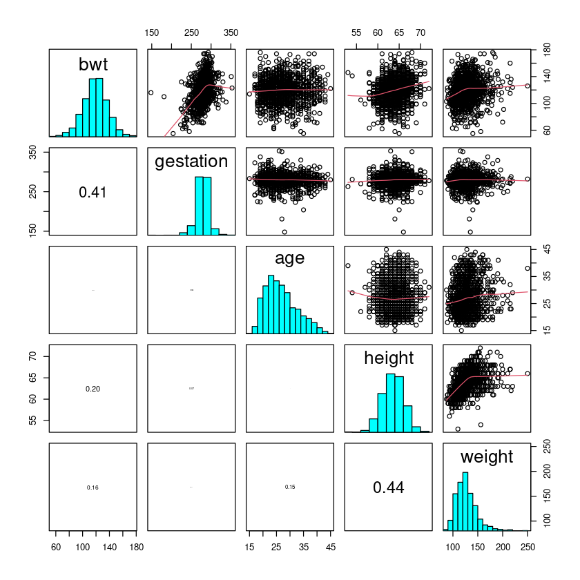
Let us first inspect the relationships between the numerical explanatory variables and the response variable.
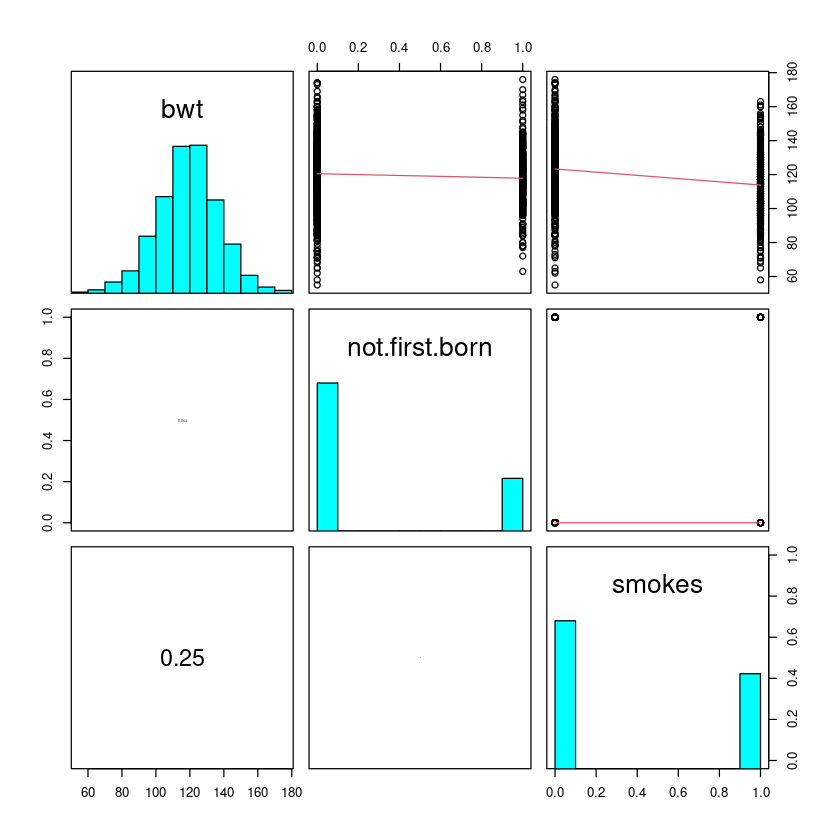
The five variables are in columns 1,2,4,5 and 6 in the data frame Babies.df.
## Invoke the s20x library
library(s20x)
## Importing data into R
Babies.df <- read.table("../data/babies_data.txt", header = T)
## Create the pairs plot of the five numeric variables
pairs20x(Babies.df[, c(1, 2, 4, 5, 6)])
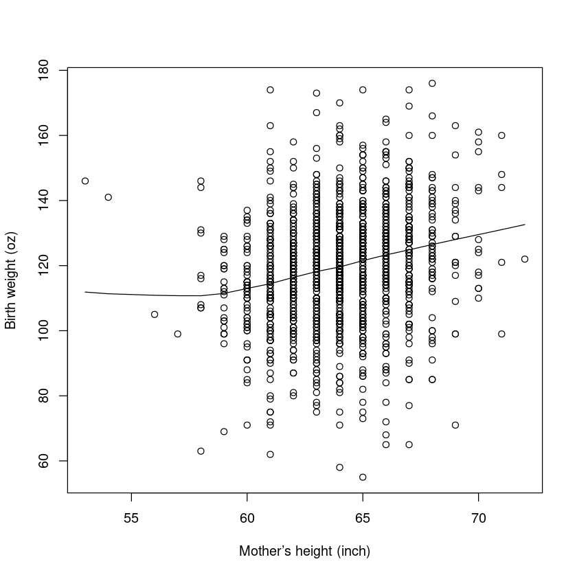
plot(bwt ~ height,
    data = Babies.df,
    xlab = "Mother’s height (inch)", ylab = "Birth weight (oz)"
)
lines(lowess(Babies.df$height, Babies.df$bwt))
summary(lm(bwt ~ height, data = Babies.df))$r.squared
cor(Babies.df$bwt, Babies.df$height)^2 # R 方是差异的平方,所以跟上边那个是一样的
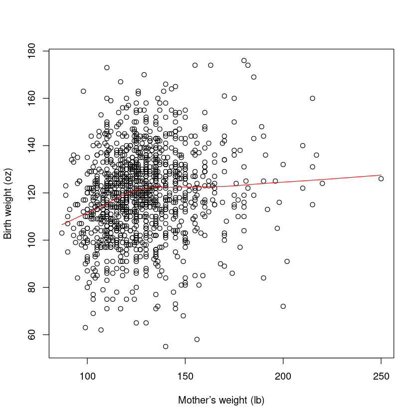
Looking at the pairs plot again, we also see a somewhat weak relationship between bwt and mother’s weight.
plot(bwt ~ weight,
    data = Babies.df,
    xlab = "Mother’s weight (lb)",
    ylab = "Birth weight (oz)"
)
lines(lowess(Babies.df$weight, Babies.df$bwt), col = "red")
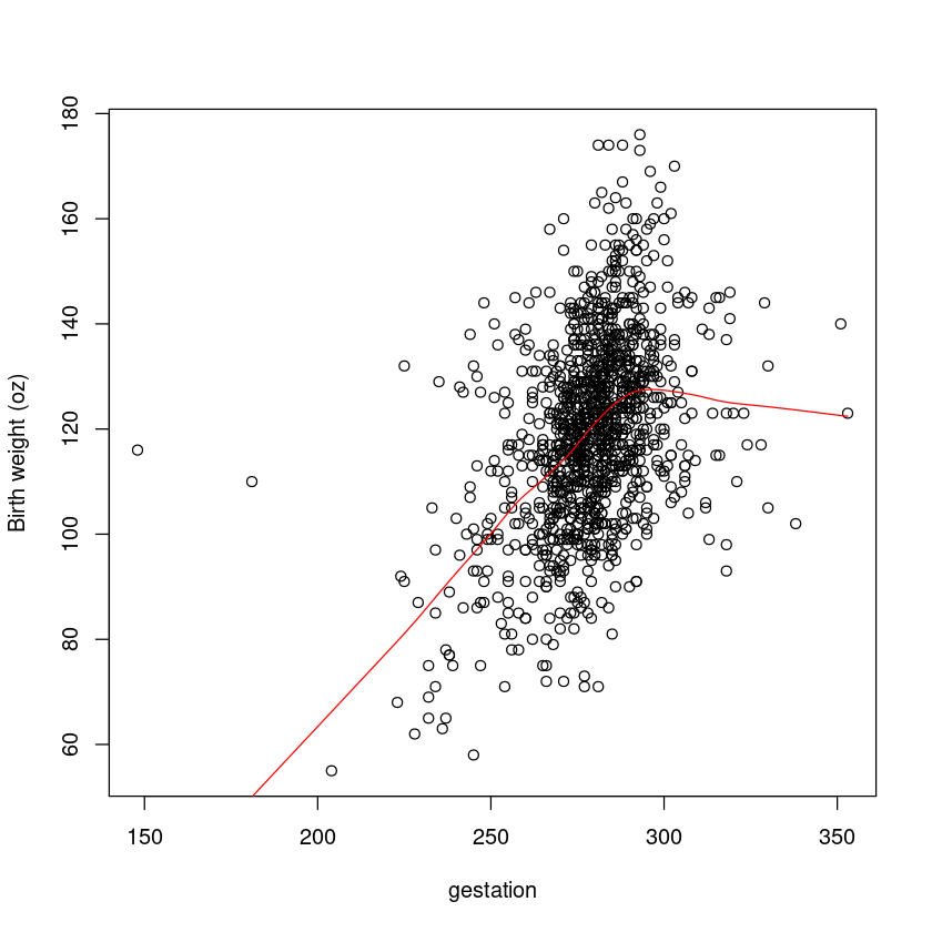
胎儿孕育时间与其出生体重之间存在更强的关系,这并不令人意外,因为孩子在母亲子宫内的时间越长,孩子就有更多的时间来获得营养和生长。但是,在某个特定的胎龄后,这种关系显然会变得平缓起来 - 有些人称其为“曲棍球杆形状的曲线”。
plot(bwt ~ gestation, data = Babies.df, ylab = "Birth weight (oz)")
lines(lowess(Babies.df$gestation, Babies.df$bwt), col = "red")
There does not seem to be any relationship between a mother’s age and her child’s bwt.
plot(bwt ~ age,
    data = Babies.df,
    xlab = "Mother’s age",
    ylab = "Birth weight (oz)"
)
lines(lowess(Babies.df$age, Babies.df$bwt), col = "red")
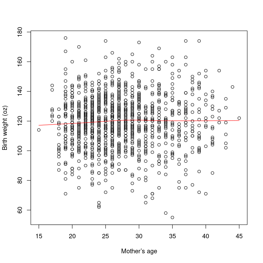
Note: There seem to be some outlying data points(一些偏远的数据点) in these plots. There does not appear to be much of a relationship between the x variables, except between height and weight.
pairs20x(Babies.df[, c(1, 3, 7)])
让我们从理解“解释”的角度开始,因为它是最强大的关系之一。那些不典型的数据点已经用问号标记了。我们稍后会添加其他的解释变量。
plot(bwt ~ gestation, data = Babies.df, ylab = "Birth weight (oz)")
lines(lowess(Babies.df$gestation, Babies.df$bwt), col = "red")
text(c(152, 185), c(120, 115), "?", col = "red")
abline(v = 294, lty = 3)
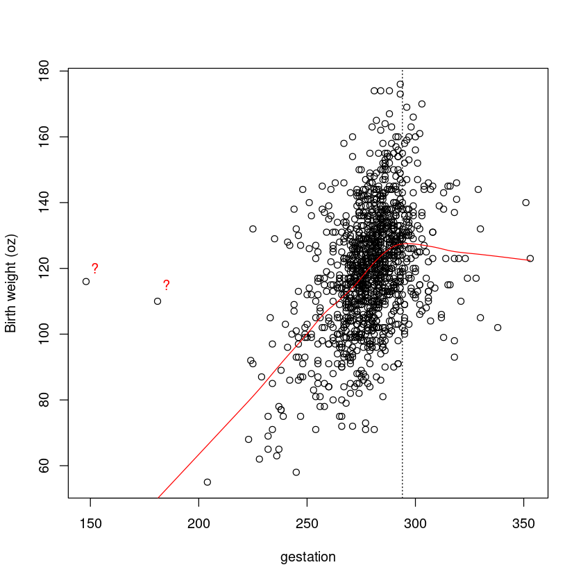
They look extremely implausible as they have typical birth-weight but have a gestational age that is extremely low for these data. 他们看起来非常难以置信,因为他们典型的出生体重但有孕龄,对这些数据是极低的。
id <- (Babies.df$gestation < 200)
Babies.df[id, ]
| bwt | gestation | not.first.born | age | height | weight | smokes | |
|---|---|---|---|---|---|---|---|
| <int> | <int> | <int> | <int> | <int> | <int> | <int> | |
| 239 | 116 | 148 | 0 | 28 | 66 | 135 | 0 |
| 820 | 110 | 181 | 0 | 27 | 64 | 133 | 0 |
Relationship between birth weight and gestational age...
For gestation \(\leq 294\) days we’ll use the familiar simple linear regression model
We’d like to extend this model by adding an extra term so that the slope changes when gestation \(> 294\). That is,
where v is some suitable explanatory variable. What should v be?
For
gestation\(\leq 294\) the extended model is just the simple linear regression model, so that means v = 0 when gestation ≤ 294.For
gestation\(> 294\) we need another slope effect for gestational age. In fact, we need \(v =\)gestation\(- 294\).
Let’s create the new explanatory v = 294 that is described gestation above. We’ll give it the name because it is the number of days ODdays that the baby is overdue.
Babies.df$ODdays <- ifelse(
    Babies.df$gestation < 294,
    0,
    Babies.df$gestation - 294
)
head(Babies.df, 12) # Print first 12 lines of dataframe
| bwt | gestation | not.first.born | age | height | weight | smokes | ODdays | |
|---|---|---|---|---|---|---|---|---|
| <int> | <int> | <int> | <int> | <int> | <int> | <int> | <dbl> | |
| 1 | 120 | 284 | 0 | 27 | 62 | 100 | 0 | 0 |
| 2 | 113 | 282 | 0 | 33 | 64 | 135 | 0 | 0 |
| 3 | 128 | 279 | 0 | 28 | 64 | 115 | 1 | 0 |
| 4 | 108 | 282 | 0 | 23 | 67 | 125 | 1 | 0 |
| 5 | 136 | 286 | 0 | 25 | 62 | 93 | 0 | 0 |
| 6 | 138 | 244 | 0 | 33 | 62 | 178 | 0 | 0 |
| 7 | 132 | 245 | 0 | 23 | 65 | 140 | 0 | 0 |
| 8 | 120 | 289 | 0 | 25 | 62 | 125 | 0 | 0 |
| 9 | 143 | 299 | 0 | 30 | 66 | 136 | 1 | 5 |
| 10 | 140 | 351 | 0 | 27 | 68 | 120 | 0 | 57 |
| 11 | 144 | 282 | 0 | 32 | 64 | 124 | 1 | 0 |
| 12 | 141 | 279 | 0 | 23 | 63 | 128 | 1 | 0 |
10.3. Fitting the initial model#
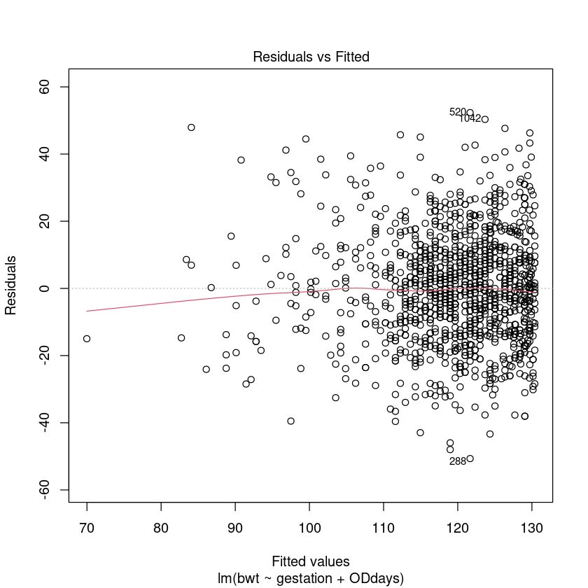
bwt.fit <- lm(bwt ~ gestation + ODdays, data = Babies.df)
plot(bwt.fit, which = 1, add.smooth = FALSE)
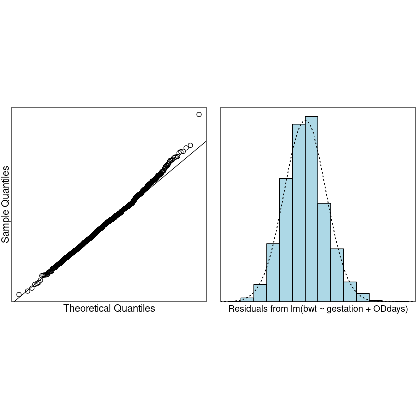
normcheck(bwt.fit)
cooks20x(bwt.fit)
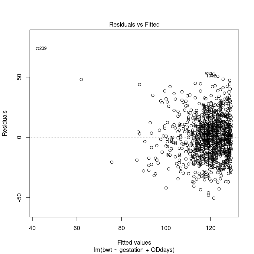
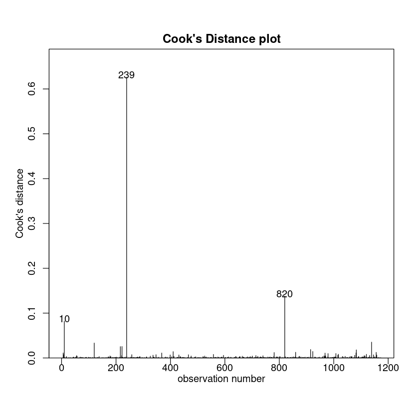
Let us refit with observation 239 removed.
bwt.fit2 <- lm(bwt ~ gestation + ODdays, data = Babies.df[-239, ])
cooks20x(bwt.fit2)
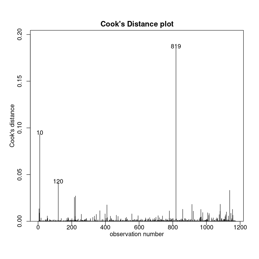
We refit the model using the reduced data.
# This time we demonstrate using the subset argument to remove points
bwt.fit3 <- lm(bwt ~ gestation + ODdays,
    data = Babies.df,
    subset = -c(239, 820)
)
cooks20x(bwt.fit3)
plot(bwt.fit3, which = 1)
Let’s take a look at our fitted hockey stick model.
gestation.seq <- 201:360 # Explanatory values at which to get predictions
ODdays.seq <- ifelse(gestation.seq <= 294, 0, gestation.seq - 294)
fit.seq <- predict(bwt.fit3, new = data.frame(
    gestation = gestation.seq,
    ODdays = ODdays.seq
))
plot(bwt ~ gestation,
    data = Babies.df[-c(239, 820), ],
    ylab = "Birth weight (oz)"
)
lines(gestation.seq, fit.seq, col = "red")
abline(v = 294, lty = 2, col = "blue")
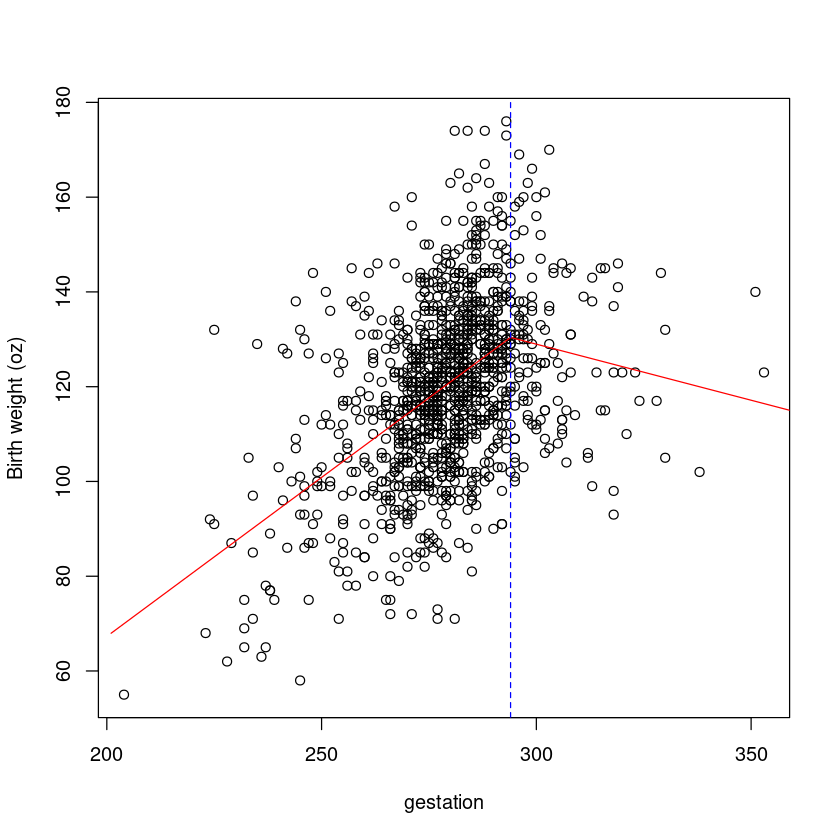
模型检查是好的,没有影响力的点依然存在,所以我们可以相信这个。让我们解释输出。
summary(bwt.fit3)
Call:
lm(formula = bwt ~ gestation + ODdays, data = Babies.df, subset = -c(239,
    820))

Residuals:
    Min      1Q  Median      3Q     Max
-50.664 -10.993  -0.308   9.795  52.336

Coefficients:
             Estimate Std. Error t value Pr(>|t|)
(Intercept) -66.95336   10.42810   -6.42 1.97e-10 ***
gestation     0.67124    0.03757   17.87  < 2e-16 ***
ODdays       -0.90783    0.11745   -7.73 2.31e-14 ***
---
Signif. codes:  0 ‘***’ 0.001 ‘**’ 0.01 ‘*’ 0.05 ‘.’ 0.1 ‘ ’ 1

Residual standard error: 16.23 on 1169 degrees of freedom
Multiple R-squared:  0.2188,	Adjusted R-squared:  0.2174
F-statistic: 163.7 on 2 and 1169 DF,  p-value: < 2.2e-16
The fitted model is:
10.4. Multiple linear regression model: Adding more terms to the model and the peril of multi-collinearity#
bwt.fit4 = lm(bwt ~ gestation + ODdays + height,
    data = Babies.df,
    subset = -c(239, 820)
)
plot(bwt.fit4, which = 1)
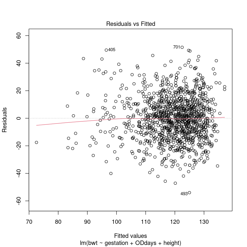
All seems okay. Let us make sure that this makes sense in terms of output.
summary(bwt.fit4)
Call:
lm(formula = bwt ~ gestation + ODdays + height, data = Babies.df,
    subset = -c(239, 820))

Residuals:
    Min      1Q  Median      3Q     Max
-53.999 -10.393  -0.050   9.772  51.514

Coefficients:
              Estimate Std. Error t value Pr(>|t|)
(Intercept) -139.20571   15.05961  -9.244  < 2e-16 ***
gestation      0.65219    0.03703  17.613  < 2e-16 ***
ODdays        -0.89039    0.11543  -7.714 2.61e-14 ***
height         1.21083    0.18495   6.547 8.79e-11 ***
---
Signif. codes:  0 ‘***’ 0.001 ‘**’ 0.01 ‘*’ 0.05 ‘.’ 0.1 ‘ ’ 1

Residual standard error: 15.94 on 1168 degrees of freedom
Multiple R-squared:  0.2464,	Adjusted R-squared:  0.2445
F-statistic: 127.3 on 3 and 1168 DF,  p-value: < 2.2e-16
Let us add weight to the model. We’re going to save some typing and use the `update`` function to update our model.
bwt.fit5 <- update(bwt.fit4, ~ . + weight)
summary(bwt.fit5)
Call:
lm(formula = bwt ~ gestation + ODdays + height + weight, data = Babies.df,
    subset = -c(239, 820))

Residuals:
    Min      1Q  Median      3Q     Max
-53.053 -10.540   0.121  10.076  47.746

Coefficients:
              Estimate Std. Error t value Pr(>|t|)
(Intercept) -131.68169   15.14974  -8.692  < 2e-16 ***
gestation      0.65624    0.03688  17.795  < 2e-16 ***
ODdays        -0.90868    0.11502  -7.900 6.41e-15 ***
height         0.90486    0.20453   4.424 1.06e-05 ***
weight         0.08535    0.02485   3.434 0.000615 ***
---
Signif. codes:  0 ‘***’ 0.001 ‘**’ 0.01 ‘*’ 0.05 ‘.’ 0.1 ‘ ’ 1

Residual standard error: 15.87 on 1167 degrees of freedom
Multiple R-squared:  0.254,	Adjusted R-squared:  0.2514
F-statistic: 99.32 on 4 and 1167 DF,  p-value: < 2.2e-16