15. Modelling proportion data using the binomial distribution#
本节需要的包:
require(s20x)
Show code cell output
Loading required package: s20x
15.1. Binary (Bernoulli) data, odds and log-odds#
Here we are considering the situation where the response can only take two possible values. These might be coded in the form of:
Zeros or ones.
TRUE or FALSE.
Yes or No.
Success or Failure.
Or any other pair of categorical values.
Bernoulli random variables(伯努利随机变量):
If Y is a Bernoulli random variable with parameter p, then Y will take the value 1 with probability p, and the value 0 with probability 1 - p. Since it is a probability, p must be a value that is between 0 and 1, i.e. \(p ∈ [0, 1]\).
很容易表明,伯努利随机变量的平均值为:
而且,方差为
15.1.1. Odds#
为了使 glm 对数几率的解释更加容易,我们需要引入 Odds 这个概念,把定义域从 \([0, 1]\) 扩展到 \([0, \infty]\)。
Odds 是指事件发生的概率与事件不发生的概率的比值,即:
反过来说:
15.1.2. Log-odds#
Odds 的对数(简称为 log-odds)为:
此时定义域从 \([0, \infty]\) 变为 \([-\infty, \infty]\)。
15.2. Modelling log-odds#
Why log-odds?
由于我们的模型对或的值没有限制,所以在设置变量为 \(β_0\)、\(β_1\) 的情况下,\(β_0 + β_1 x\) 可以在实线上取任何值。
That is, \(\beta_0+\beta_1x\in(-\infty,\infty)\).
Log-Odds can be any real number.
即:
其中p是解释变量x的主体 "成功" 的概率。
This can be re-arranged in the logistic form
15.3. Modelling the response when it is binary (ungrouped data) via glm#
bb.df <- read.csv("../data/basketball.csv")
head(bb.df, 10)
| distance | gender | basket | |
|---|---|---|---|
| <int> | <chr> | <int> | |
| 1 | 3 | M | 1 |
| 2 | 1 | F | 1 |
| 3 | 2 | M | 1 |
| 4 | 3 | M | 0 |
| 5 | 1 | M | 1 |
| 6 | 2 | F | 1 |
| 7 | 2 | F | 1 |
| 8 | 1 | F | 1 |
| 9 | 3 | F | 0 |
| 10 | 1 | F | 1 |
success.tbl <- xtabs(basket ~ distance + gender, data = bb.df)
success.tbl
        gender
distance  F  M
       1 10 10
       2  6  5
       3  2  1
bb.fit <- glm(
    basket ~ distance * gender,
    family = binomial, # binomial distribution
    data = bb.df
)
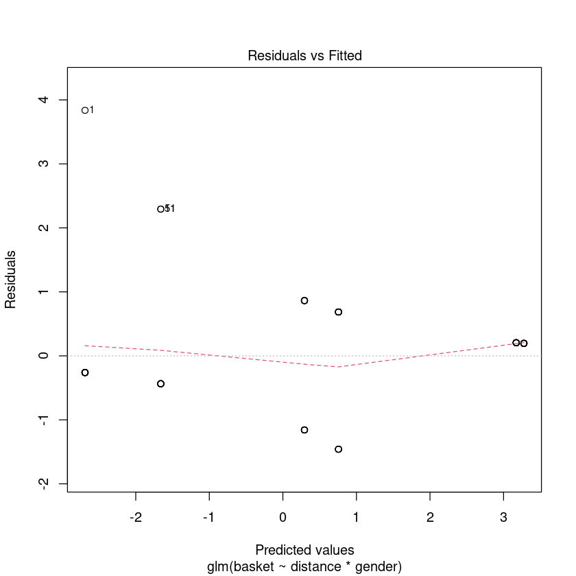
plot(bb.fit, which = 1, lty = 2)
summary(bb.fit)
Call:
glm(formula = basket ~ distance * gender, family = binomial,
    data = bb.df)

Deviance Residuals:
    Min       1Q   Median       3Q      Max
-1.5106  -0.5900   0.2723   0.2866   2.3474

Coefficients:
                 Estimate Std. Error z value Pr(>|z|)
(Intercept)        5.5878     1.9050   2.933  0.00335 **
distance          -2.4159     0.8181  -2.953  0.00314 **
genderM            0.6710     2.9235   0.230  0.81847
distance:genderM  -0.5668     1.3213  -0.429  0.66794
---
Signif. codes:  0 ‘***’ 0.001 ‘**’ 0.01 ‘*’ 0.05 ‘.’ 0.1 ‘ ’ 1

(Dispersion parameter for binomial family taken to be 1)

    Null deviance: 82.108  on 59  degrees of freedom
Residual deviance: 46.202  on 56  degrees of freedom
AIC: 54.202

Number of Fisher Scoring iterations: 5
bb.fit1 <- glm(basket ~ distance + gender,
    family = binomial, data = bb.df
)
summary(bb.fit1)
Call:
glm(formula = basket ~ distance + gender, family = binomial,
    data = bb.df)

Deviance Residuals:
    Min       1Q   Median       3Q      Max
-1.5382  -0.5411   0.2461   0.3219   2.2283

Coefficients:
            Estimate Std. Error z value Pr(>|z|)
(Intercept)   6.1469     1.5242   4.033 5.51e-05 ***
distance     -2.6648     0.6364  -4.188 2.82e-05 ***
genderM      -0.5478     0.7486  -0.732    0.464
---
Signif. codes:  0 ‘***’ 0.001 ‘**’ 0.01 ‘*’ 0.05 ‘.’ 0.1 ‘ ’ 1

(Dispersion parameter for binomial family taken to be 1)

    Null deviance: 82.108  on 59  degrees of freedom
Residual deviance: 46.392  on 57  degrees of freedom
AIC: 52.392

Number of Fisher Scoring iterations: 5
bb.fit2 <- glm(basket ~ distance, family = binomial, data = bb.df)
summary(bb.fit2)
Call:
glm(formula = basket ~ distance, family = binomial, data = bb.df)

Deviance Residuals:
    Min       1Q   Median       3Q      Max
-1.4118  -0.4818   0.2873   0.2873   2.1029

Coefficients:
            Estimate Std. Error z value Pr(>|z|)
(Intercept)   5.7980     1.4038   4.130 3.63e-05 ***
distance     -2.6310     0.6274  -4.193 2.75e-05 ***
---
Signif. codes:  0 ‘***’ 0.001 ‘**’ 0.01 ‘*’ 0.05 ‘.’ 0.1 ‘ ’ 1

(Dispersion parameter for binomial family taken to be 1)

    Null deviance: 82.108  on 59  degrees of freedom
Residual deviance: 46.937  on 58  degrees of freedom
AIC: 50.937

Number of Fisher Scoring iterations: 5
coef(bb.fit2)
- (Intercept)
- 5.79796774980361
- distance
- -2.63103340427345
exp(coef(bb.fit2))
100 * (1 - exp(coef(bb.fit2)))
- (Intercept)
- 329.628990177678
- distance
- 0.0720040145217848
- (Intercept)
- -32862.8990177678
- distance
- 92.7995985478215
(bb.ci2 <- confint(bb.fit2))
100 * (1 - exp(bb.ci2))
Waiting for profiling to be done...
| 2.5 % | 97.5 % | |
|---|---|---|
| (Intercept) | 3.422396 | 9.037020 |
| distance | -4.103523 | -1.568945 |
| 2.5 % | 97.5 % | |
|---|---|---|
| (Intercept) | -2964.27509 | -840767.86136 |
| distance | 98.34856 | 79.17351 |
predn.df <- data.frame(distance = 1:3)
bb.logit.pred <- predict(bb.fit2, newdata = predn.df)
bb.logit.pred
- 1
- 3.16693434553016
- 2
- 0.53590094125671
- 3
- -2.09513246301674
plogis(bb.logit.pred)
- 1
- 0.959570820970203
- 2
- 0.630858358052515
- 3
- 0.109570820976233
predict(bb.fit2, newdata = predn.df, type = "response")
- 1
- 0.959570820970203
- 2
- 0.630858358052515
- 3
- 0.109570820976233
bb.logit.predses <- predict(bb.fit2, newdata = predn.df, se.fit = TRUE)$se.fit
bb.logit.predses
# Lower and upper bounds of CIs for the log-odds
lower = bb.logit.pred - 1.96 * bb.logit.predses
upper = bb.logit.pred + 1.96 * bb.logit.predses
ci = cbind(lower, upper)
plogis(ci)
- 1
- 0.815101808705842
- 2
- 0.381297733450052
- 3
- 0.643231168633725
| lower | upper | |
|---|---|---|
| 1 | 0.82768876 | 0.9915452 |
| 2 | 0.44733541 | 0.7830016 |
| 3 | 0.03370361 | 0.3027157 |
predictGLM(bb.fit2, newdata = data.frame(distance = 1:3), type = "link")
predictGLM(bb.fit2, newdata = data.frame(distance = 1:3), type = "response")
***Estimates and CIs are on the link scale***
| fit | lwr | upr | |
|---|---|---|---|
| 1 | 3.1669343 | 1.5693642 | 4.7645045 |
| 2 | 0.5359009 | -0.2114289 | 1.2832308 |
| 3 | -2.0951325 | -3.3558424 | -0.8344225 |
***Estimates and CIs are on the response scale***
| fit | lwr | upr | |
|---|---|---|---|
| 1 | 0.9595708 | 0.82769294 | 0.9915450 |
| 2 | 0.6308584 | 0.44733881 | 0.7829992 |
| 3 | 0.1095708 | 0.03370437 | 0.3027108 |
15.4. Modelling the response when it is binomial (grouped binary data) via glm#
# Load dplyr package to manipulate data frames
library(dplyr)
bb.grouped.df = bb.df %>%
    group_by(gender, distance) %>%
    summarize(n = n(), propn = sum(basket) / n)
# Change tibble back to a data frame
bb.grouped.df = data.frame(bb.grouped.df)
bb.grouped.df
Error in library(dplyr): there is no package called ‘dplyr’
Traceback:

1. library(dplyr)
这样转换后,虽然结果相同,但我们可以做卡方检验了(手动经历了分组)。
bb.fit3 = glm(propn ~ distance * gender,
    weights = n,
    family = binomial, data = bb.grouped.df
)
summary(bb.fit3)
Call:
glm(formula = propn ~ distance * gender, family = binomial, data = bb.grouped.df,
    weights = n)

Deviance Residuals:
      1        2        3        4        5        6
 0.9063  -0.5354   0.3367   0.8612  -0.4629   0.4376

Coefficients:
                 Estimate Std. Error z value Pr(>|z|)
(Intercept)        5.5878     1.9050   2.933  0.00335 **
distance          -2.4159     0.8181  -2.953  0.00314 **
genderM            0.6710     2.9236   0.230  0.81848
distance:genderM  -0.5668     1.3214  -0.429  0.66795
---
Signif. codes:  0 '***' 0.001 '**' 0.01 '*' 0.05 '.' 0.1 ' ' 1

(Dispersion parameter for binomial family taken to be 1)

    Null deviance: 38.2749  on 5  degrees of freedom
Residual deviance:  2.3688  on 2  degrees of freedom
AIC: 20.23

Number of Fisher Scoring iterations: 4
1 - pchisq(2.3688, 2)
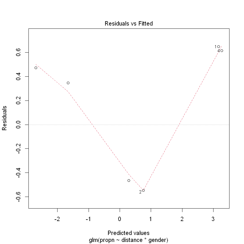
plot(bb.fit3, which = 1, lty = 2)
bb.grouped.df <- transform(bb.grouped.df, success = n * propn, fail = n * (1 - propn))
bb.grouped.df
| gender | distance | n | propn | success | fail |
|---|---|---|---|---|---|
| <chr> | <int> | <int> | <dbl> | <dbl> | <dbl> |
| F | 1 | 10 | 1.0 | 10 | 0 |
| F | 2 | 10 | 0.6 | 6 | 4 |
| F | 3 | 10 | 0.2 | 2 | 8 |
| M | 1 | 10 | 1.0 | 10 | 0 |
| M | 2 | 10 | 0.5 | 5 | 5 |
| M | 3 | 10 | 0.1 | 1 | 9 |
bb.fit4 = glm(cbind(success, fail) ~ distance * gender,
    family = binomial,
    data = bb.grouped.df
)
summary(bb.fit4)
15.5. Example 1: Space shuttle Challenger accident#
The NASA space shuttle Challenger broke up during launch on the cold morning of 28 January 1986. Most of the crew survived the initial break-up, but are believed to have been killed when the crew capsule hit the ocean at high speed. 1986年1月28日的寒冷早晨,美国宇航局的挑战者号航天飞机在发射过程中解体。大多数机组人员在最初的解体过程中幸存下来,但据信在机组人员舱高速撞向海洋时被杀死。
Space.df <- read.table("../data/ChallengerShuttle.txt", head = TRUE)
Space.df$Temp
Space.df$Failure
- 66
- 70
- 69
- 68
- 67
- 72
- 73
- 70
- 57
- 63
- 70
- 78
- 67
- 53
- 67
- 75
- 70
- 81
- 76
- 79
- 75
- 76
- 58
- 0
- 1
- 0
- 0
- 0
- 0
- 0
- 0
- 1
- 1
- 1
- 0
- 0
- 2
- 0
- 0
- 0
- 0
- 0
- 0
- 2
- 0
- 1
Space.gfit = glm(cbind(Failure, 6 - Failure) ~ Temp,
    family = binomial,
    data = Space.df
)
summary(Space.gfit)
Call:
glm(formula = cbind(Failure, 6 - Failure) ~ Temp, family = binomial,
    data = Space.df)

Deviance Residuals:
     Min        1Q    Median        3Q       Max
-0.95227  -0.78299  -0.54117  -0.04379   2.65152

Coefficients:
            Estimate Std. Error z value Pr(>|z|)
(Intercept)  5.08498    3.05247   1.666   0.0957 .
Temp        -0.11560    0.04702  -2.458   0.0140 *
---
Signif. codes:  0 '***' 0.001 '**' 0.01 '*' 0.05 '.' 0.1 ' ' 1

(Dispersion parameter for binomial family taken to be 1)

    Null deviance: 24.230  on 22  degrees of freedom
Residual deviance: 18.086  on 21  degrees of freedom
AIC: 35.647

Number of Fisher Scoring iterations: 5
predictGLM(Space.gfit, newdata = data.frame(Temp = 31), type = "response")
6 * predictGLM(Space.gfit, newdata = data.frame(Temp = 31), type = "response")