3. The null model#
本课程前置需要装的包:
require(s20x)
require(bootstrap)
Show code cell output
Loading required package: s20x
Loading required package: bootstrap
3.1. Revisiting the null model 回顾零模型#
本节同样以 Stats20x 的学生考试成绩为例:
Stats20x.df <- read.table("../data/STATS20x.txt", header = TRUE, sep = "\t")
零模型就是把线性模型中的斜率去掉,或斜率指定常数,从而排除其影响单独分析截距。本节将重点讲述零模型的最大作用:T检验。
t检验(t test)又称学生t检验(Student t-test)可以说是统计推断中非常常见的一种检验方法,用于统计量服从正态分布,但方差未知的情况。
t检验的前提是要求样本服从正态分布或近似正态分布,不然可以利用一些变换(取对数、开根号、倒数等等)试图将其转化为服从正态分布是数据,如若还是不满足正态分布,只能利用非参数检验方法。不过当样本量大于30的时候,可以认为数据近似正态分布。
t检验最常见的四个用途:
单样本均值检验(One-sample t-test) 用于检验 “总体方差未知、正态数据或近似正态的” 单样本的均值,是否与已知的总体均值相等。
两独立样本均值检验(Independent two-sample t-test) 用于检验两对 “独立的,正态数据或近似正态的” 样本的均值是否相等,这里可根据总体方差是否相等分类讨论。
配对样本均值检验(Dependent t-test for paired samples) 用于检验一对配对样本的均值的差,是否等于某一个值
回归系数的显著性检验(t-test for regression coefficient significance) 用于检验回归模型的解释变量,对被解释变量是否有显著影响
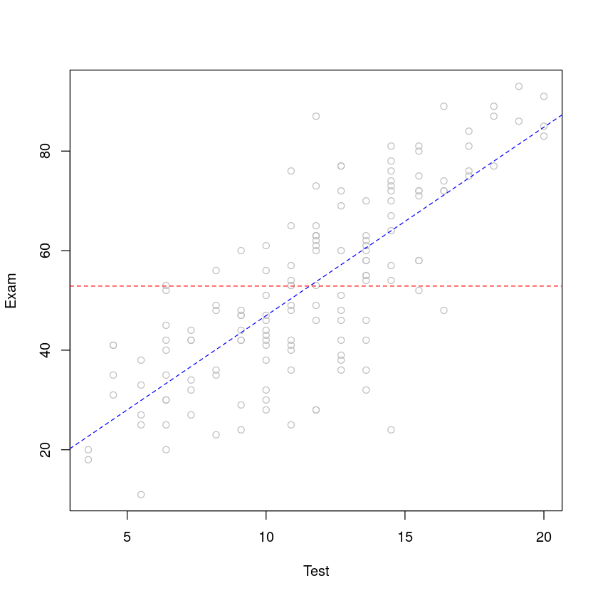
# 建立回归模型
examtest.fit <- lm(Exam ~ Test, data = Stats20x.df)
examtest.fit2 <- lm(Exam ~ 1, data = Stats20x.df)

# 绘图
plot(Exam ~ Test, data = Stats20x.df, col = "grey")
abline(examtest.fit, col = "blue", lty = 2)
abline(examtest.fit2, col = "red", lty = 2)
推断总体均值:
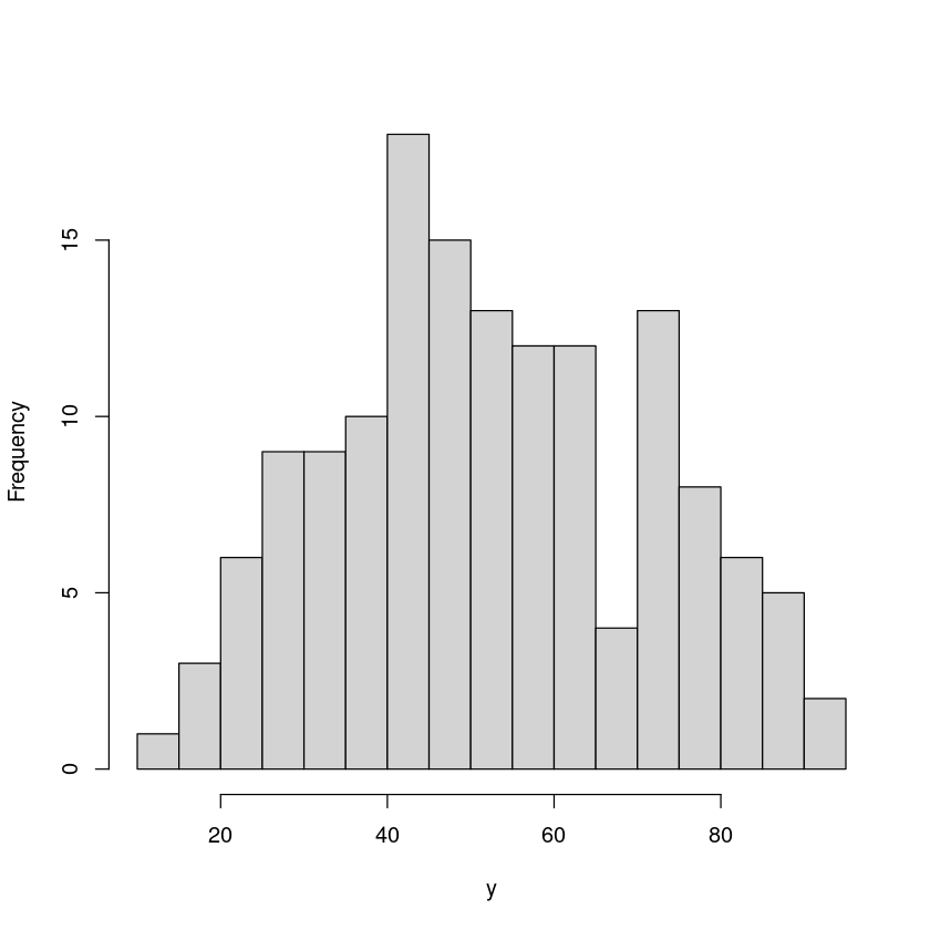
To save some typing we’ll let y be the vector Stats20x.df$Exam of exam scores.
y <- Stats20x.df$Exam
hist(y, breaks = 20, main = "") # Use main to suppress plot title
继续使用零模型做线性回归,使其更关注于y值的置信关系与p检验。
null.fit <- lm(y ~ 1)
# Only give coefficients from summary 将系数板块单独提取出做展示
coef(summary(null.fit))
# 获得该零模型的对应置信区间
confint(null.fit)
| Estimate | Std. Error | t value | Pr(>|t|) | |
|---|---|---|---|---|
| (Intercept) | 52.87671 | 1.545802 | 34.20666 | 2.632011e-71 |
| 2.5 % | 97.5 % | |
|---|---|---|
| (Intercept) | 49.8215 | 55.93193 |
Conclusion:
The near zero \(Pr(>|t|)\) p-value totally rejects(拒绝) the null hypothesis(零假设) that \(H0 : µ ≡ β0 = 0\).
The 95% confidence interval(置信区间) for \(µ\) is 49.82 to 55.93.
3.2. Revisiting the t-test#
其中 \(\bar{y}\) 为样本均值,\(s\) 为样本标准差。
n <- length(y) # 146 students
tstat <- (mean(y) - 0) / (sd(y) / sqrt(n))
tstat
## t-multiplier
tmult <- qt(1 - .05 / 2, df = n - 1)
## We want the upper 97.5% (or 1-.05/2) bound of the CI
## NOTE: mean = sample mean; sd = standard deviation; sqrt = square root
mean(y) - tmult * sd(y) / sqrt(n)

## Upper bound of CI 置信区间上限
mean(y) + tmult * sd(y) / sqrt(n)
## Or if we want both the lower and upper bounds of the CI in one statement
## 置信区间下限
mean(y) + c(-1, 1) * tmult * sd(y) / sqrt(n)
- 49.8214976403875
- 55.9319270171467
零模型就是单样本T检验。
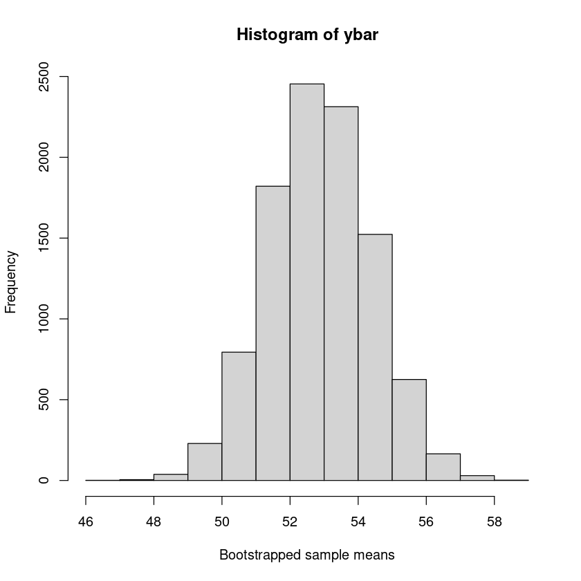
手动随机抽样检验我们的结果:
## Resampling the exam marks, N times with replacement:
N <- 10000 # The number of bootstrap resamples we want
# The new sample means are stored in ybar
ybar <- rep(NA, N) ## A vector of length N to store our resampled means

## A loop - allows us to do something N (10,000) times
for (i in 1:N) {
    ## Take the average of this sample (below) from a sample of size n = 146 from y - with replacement
    ybar[i] <- mean(sample(y, n, replace = T))
}
mean(ybar)
library(bootstrap)
ybar <- bootstrap(Stats20x.df$Exam, 10000, mean)$thetastar
mean(ybar)
## Histogram of these 10,000 bootstrap means
hist(ybar, xlab = "Bootstrapped sample means")
3.3. The paired t-test#
For a meaningful comparison, We will need to make them have the same scale, so we multiply the test mark by 5 so that it is also out of 100.
Stats20x.df$Test2 <- 5 * Stats20x.df$Test
## Check that it worked
Stats20x.df[1:3, c("Exam", "Test", "Test2")]
| Exam | Test | Test2 | |
|---|---|---|---|
| <int> | <dbl> | <dbl> | |
| 1 | 42 | 9.1 | 45.5 |
| 2 | 58 | 13.6 | 68.0 |
| 3 | 81 | 14.5 | 72.5 |
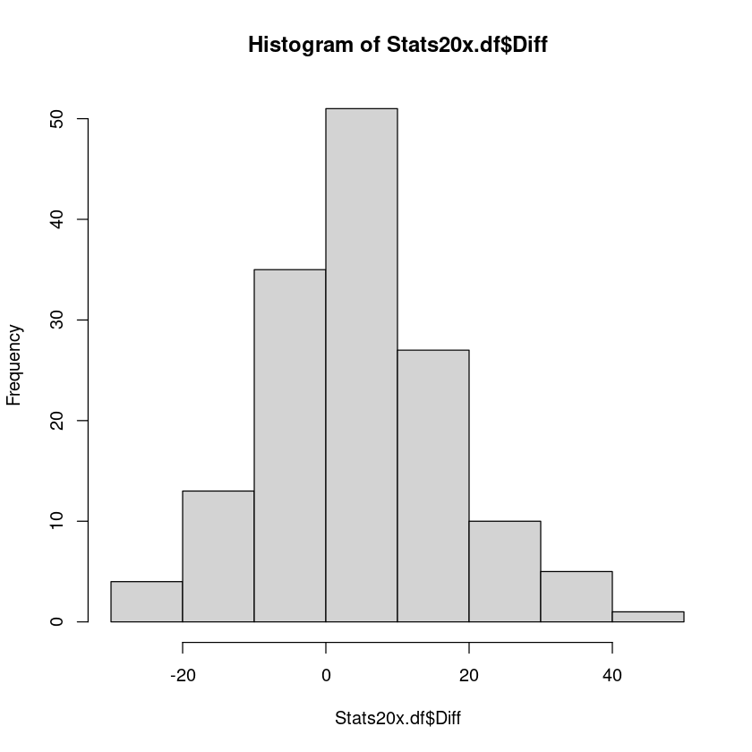
Stats20x.df$Diff <- Stats20x.df$Test2 - Stats20x.df$Exam
## Check the first 5 measurements
Stats20x.df[1:5, c("Test2", "Exam", "Diff")]
| Test2 | Exam | Diff | |
|---|---|---|---|
| <dbl> | <int> | <dbl> | |
| 1 | 45.5 | 42 | 3.5 |
| 2 | 68.0 | 58 | 10.0 |
| 3 | 72.5 | 81 | -8.5 |
| 4 | 95.5 | 86 | 9.5 |
| 5 | 41.0 | 35 | 6.0 |
hist(Stats20x.df$Diff)